Finite Element Analysis Explained

What is Finite Element Analysis (FEA)?

Finite Element Analysis (FEA) is a sophisticated numerical method used by engineers to predict how a product, component, or structure reacts to various physical forces, such as stress, heat, vibration, and fluid flow. Essentially, it allows for the simulation of real-world physical phenomena within a virtual environment. The fundamental concept behind FEA is to break down a complex object into a multitude of smaller, simpler parts, known as “finite elements.” These elements, which can be triangles, quadrilaterals, tetrahedrons, or bricks, are interconnected at specific points called “nodes.” By analyzing the behavior of each individual element and then reassembling them, engineers can obtain an approximate solution for the entire complex structure.

Historically, solving complex engineering problems often relied on analytical methods, which are precise but only applicable to simple geometries and load conditions. For intricate designs or non-linear material behaviors, these methods quickly become intractable. This is where FEA steps in, offering a robust solution for problems that are impossible or impractical to solve manually. It transforms complex differential equations that govern physical behavior into a system of algebraic equations that can be solved by computers. The power of FEA lies in its ability to handle arbitrary geometries, diverse material properties (isotropic, anisotropic, viscoelastic, etc.), and a wide range of boundary conditions and loading scenarios, making it an incredibly versatile tool across virtually all engineering disciplines.

The origins of FEA can be traced back to the aerospace industry in the mid-20th century, driven by the need to analyze complex aircraft structures efficiently. Since then, advancements in computational power and algorithmic sophistication have propelled FEA from a specialized tool to an industry standard. Today, it is an integral part of product development, enabling engineers to virtually test and refine designs, predict potential failures, optimize performance, and reduce the need for expensive and time-consuming physical prototypes. For a manufacturing powerhouse like Mitsubishi, the ability to conduct virtual testing with high fidelity means faster innovation cycles, significant cost savings, and the production of more reliable and higher-performing products.

The Core Principles and Methodology of FEA

Understanding the methodology behind FEA is key to appreciating its power and limitations. The process typically involves several distinct steps, each critical to achieving accurate and reliable simulation results. When finite element analysis is explained in detail, these steps reveal the intricate dance between geometry, physics, and computation.

1. Pre-processing: Model Creation and Discretization (Meshing)

• Geometry Definition: The process begins with creating or importing a precise 3D CAD (Computer-Aided Design) model of the component or system to be analyzed. This digital representation serves as the foundation for the simulation.
• Material Properties: Engineers must define the material properties of the component. This includes mechanical properties like Young’s modulus, Poisson’s ratio, yield strength, and ultimate tensile strength, as well as thermal properties, density, and more. The accuracy of these inputs, often derived from rigorous Materials Science In Manufacturing research and testing, is paramount for a reliable simulation.
• Meshing (Discretization): This is arguably the most crucial step in pre-processing. The continuous geometry of the model is divided into a finite number of discrete, interconnected elements. The choice of element type (e.g., beam, shell, solid) and mesh density significantly impacts both the accuracy of the results and the computational time required. A finer mesh (more elements) generally yields more accurate results but demands greater computational resources. Strategic meshing, often employing adaptive meshing techniques, aims to balance accuracy with efficiency.

2. Applying Boundary Conditions and Loads

• Boundary Conditions: These define how the model interacts with its environment. They specify constraints on the model’s movement (e.g., fixed supports, pins, rollers) or prescribed displacements.
• Loads: These represent the external forces or conditions acting on the component. Common types include concentrated forces, distributed pressures, thermal loads, accelerations, and moments. Accurately representing real-world loading conditions is vital for a meaningful simulation.

3. Solving the System of Equations

• Once the model is meshed, material properties are assigned, and boundary conditions and loads are applied, the FEA software formulates a system of algebraic equations for each element based on chosen physics principles (e.g., equilibrium equations for structural analysis, heat transfer equations for thermal analysis).
• These individual element equations are then assembled into a global system of equations that represents the entire structure.
• The software then solves this large system of equations to determine unknown primary variables, such as nodal displacements in structural analysis, temperatures in thermal analysis, or velocities in fluid dynamics. This step requires significant computational power, especially for large, complex models or transient analyses.

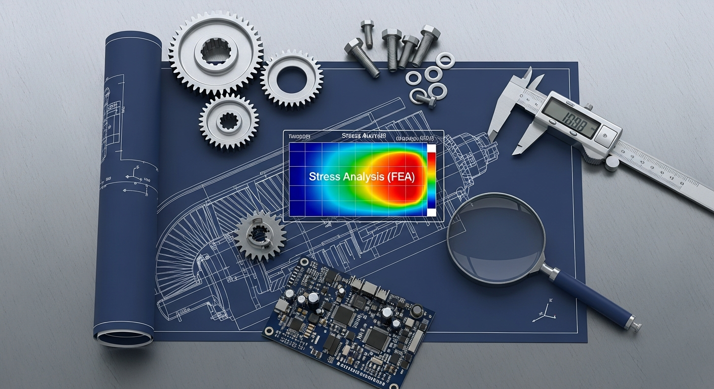
4. Post-processing: Interpreting Results

• The raw numerical results (e.g., nodal displacements) are then processed and visualized in an understandable format.
• Engineers can view stress distributions, strain patterns, deformations, temperature gradients, and other critical output variables through color contour plots, animations, graphs, and tables.
• This step allows for detailed analysis and interpretation, helping engineers identify critical areas of stress concentration, predict failure points, assess performance, and make informed design decisions. Effective post-processing is crucial for translating complex data into actionable insights for manufacturing improvements.

The iterative nature of FEA means that engineers often go back and forth between these steps, refining the model, adjusting parameters, and re-running simulations until optimal design solutions are achieved. This rigorous methodology underpins the reliability and predictive power of FEA, making it an indispensable tool for Mitsubishi Manufacturing in developing robust and innovative products.

Why FEA is Indispensable in Modern Manufacturing

One of the most significant advantages of FEA is its ability to reduce the need for physical prototyping and testing. Traditionally, designing a new component involved creating multiple physical prototypes, testing them under various conditions, identifying flaws, redesigning, and repeating the process. This cycle is incredibly time-consuming, expensive, and resource-intensive. With FEA, engineers can perform thousands of virtual tests on a digital prototype, identifying and rectifying design weaknesses before any material is cut or molded. This virtual validation process dramatically cuts down on material waste, labor costs, and the time-to-market, which are central tenets of effective Manufacturing Waste Reduction Strategies.

Furthermore, FEA directly supports the implementation of Lean Manufacturing Principles Explained by minimizing waste in its various forms. By optimizing designs early in the process, FEA helps to prevent:

• Defects: Predicting potential failure modes and stress concentrations virtually reduces the likelihood of producing faulty parts.
• Overproduction: Better-validated designs mean less need for over-engineering or producing excess parts for testing.
• Waiting: Design iterations are significantly faster in a virtual environment compared to physical prototyping.
• Transportation and Inventory: Fewer physical prototypes mean less movement of materials and reduced inventory of test components.
• Motion: Less manual intervention in design validation and testing.
• Over-processing: Optimized designs often simplify manufacturing processes, reducing unnecessary steps.

This direct impact on waste reduction makes FEA a powerful enabler of Lean practices, fostering a culture of continuous improvement and efficiency within Mitsubishi Manufacturing.

Beyond waste reduction, FEA enhances product performance and reliability. By simulating extreme conditions and complex interactions, engineers can fine-tune designs to withstand harsh environments, extend product lifespan, and improve overall functionality. This leads to higher-quality products that meet or exceed customer expectations, bolstering brand reputation and reducing warranty claims. For critical components, such as those in automotive or aerospace applications, the ability to precisely predict structural integrity and fatigue life is non-negotiable for safety and operational excellence.

FEA also facilitates innovation and design exploration. Engineers are empowered to experiment with novel geometries, advanced materials, and unconventional assembly methods without the prohibitive costs associated with physical trials. This freedom to innovate allows Mitsubishi Manufacturing to explore cutting-edge solutions, develop entirely new product categories, and stay ahead of technological curves. For instance, simulating the behavior of composite materials or additively manufactured parts, which have complex anisotropic properties, would be nearly impossible without the predictive capabilities of FEA.

Finally, FEA plays a crucial role in regulatory compliance and certification. Many industries have stringent safety and performance standards that products must meet. FEA simulations can provide compelling evidence of a product’s compliance, streamlining the certification process and ensuring that Mitsubishi’s offerings adhere to the highest global standards. As manufacturing processes become more complex and material science evolves, the predictive power of FEA will only grow in importance, solidifying its status as an indispensable tool for achieving manufacturing excellence in 2026 and beyond.

Key Applications of FEA Across Industries

The versatility of Finite Element Analysis means it is not confined to a single industry but rather serves as a fundamental engineering tool across a vast spectrum of sectors. From the microscopic world of medical devices to the colossal structures of civil engineering, FEA’s ability to predict and optimize performance is invaluable. When finite element analysis is explained through its applications, its ubiquitous nature in modern engineering becomes clear.

Automotive Industry

In the automotive sector, FEA is absolutely critical. It is used extensively for:

• Crashworthiness Simulation: Predicting how vehicle structures deform and absorb energy during collisions, crucial for occupant safety.
• Chassis and Body Design: Optimizing stiffness, weight, and vibration characteristics to enhance handling, fuel efficiency, and passenger comfort.
• Engine and Powertrain Components: Analyzing thermal stress, fatigue life, and wear on parts like pistons, crankshafts, and gearboxes.
• NVH (Noise, Vibration, and Harshness) Analysis: Identifying and mitigating sources of unwanted noise and vibration to improve ride quality.

These applications allow manufacturers like Mitsubishi to design safer, lighter, and more efficient vehicles, meeting increasingly stringent regulatory and consumer demands.

Aerospace Industry

Given the extreme operating conditions and paramount safety requirements, FEA is indispensable in aerospace. It is deployed for:

• Structural Integrity: Analyzing wings, fuselages, and landing gear for stress, fatigue, and fracture mechanics under various flight loads and temperatures.
• Weight Optimization: Designing components that are as light as possible without compromising strength, directly impacting fuel efficiency.
• Thermal Management: Simulating heat distribution in engines and other critical systems.
• Vibration Analysis: Ensuring components can withstand dynamic loads and prevent resonance failures.

The use of FEA helps ensure the reliability and longevity of aircraft, rockets, and satellites.

Medical Devices

The precision and reliability required for medical implants and instruments make FEA a vital tool:

• Biocompatibility and Stress Analysis: Simulating how implants (e.g., hip replacements, dental implants, stents) interact with biological tissue and withstand physiological loads.
• Device Performance: Optimizing the design of surgical tools, drug delivery systems, and diagnostic equipment.
• Fatigue Life: Predicting the long-term durability of devices that experience repetitive loading within the human body.

FEA helps ensure patient safety and the effectiveness of medical interventions.

Consumer Goods

Even for everyday products, FEA plays a significant role in design and performance:

• Durability and Ergonomics: Analyzing the structural integrity of electronics casings, furniture, and appliances, and optimizing their ergonomic design for user comfort and safety.
• Drop Test Simulation: Predicting how products will withstand impact from accidental drops.
• Thermal Performance: Ensuring proper heat dissipation in electronic devices like laptops and smartphones.

FEA enables companies to bring more robust, user-friendly, and reliable products to market faster.

Heavy Machinery and Industrial Equipment

For large-scale industrial applications, FEA ensures the robustness and efficiency of equipment:

• Structural Analysis: Designing cranes, excavators, and manufacturing robots to handle immense loads and cyclical operations without failure.
• Fluid Dynamics: Optimizing the performance of pumps, valves, and hydraulic systems.
• Vibration Control: Mitigating vibration in large rotating machinery to extend lifespan and improve operational stability.

Mitsubishi Manufacturing, with its diverse portfolio spanning many of these sectors, heavily relies on FEA to maintain its reputation for engineering excellence and to continue innovating in 2026.

The Role of Materials Science in FEA Success

While Finite Element Analysis is a powerful computational tool, its accuracy and predictive capabilities are profoundly dependent on the quality of its inputs, particularly the material properties. This is where the critical intersection of FEA and Materials Science In Manufacturing becomes evident. The success of any FEA simulation hinges on having a deep and accurate understanding of how materials behave under various conditions. Without precise material data, even the most sophisticated FEA software can yield misleading results, undermining the entire simulation effort.

Materials science provides the fundamental knowledge about the structure, properties, processing, and performance of materials. For FEA, this translates into supplying the constitutive models that describe a material’s response to applied loads, temperature changes, and environmental factors. Key material properties essential for accurate FEA simulations include:

• Elastic Properties: Young’s Modulus (stiffness), Poisson’s Ratio (tendency to deform in directions perpendicular to the applied force), and Shear Modulus. These define a material’s elastic deformation.
• Plasticity and Yield Strength: For materials undergoing permanent deformation, understanding the yield point and post-yield behavior (stress-strain curve) is crucial for predicting failure and large deformations.
• Fatigue Properties: For components subjected to cyclical loading, fatigue strength and endurance limits are vital to predict lifespan and prevent sudden failure.
• Thermal Properties: Thermal conductivity, specific heat, and coefficient of thermal expansion are necessary for thermal stress analysis and heat transfer simulations.
• Density: Essential for calculating inertial forces in dynamic analyses and gravitational loads.
• Anisotropic Properties: For advanced materials like composites or certain additively manufactured parts, properties can vary with direction. Materials science helps characterize these complex behaviors, which FEA can then model.

The precision of FEA simulations is inextricably linked to the accuracy of these material data inputs. This highlights the profound importance of Materials Science In Manufacturing, as an in-depth understanding of material behavior under various conditions is the bedrock upon which reliable FEA models are built. Engineers and material scientists often collaborate to gather this data through extensive laboratory testing, including tensile tests, compression tests, fatigue tests, creep tests, and impact tests. Advanced characterization techniques, such as microscopy, spectroscopy, and X-ray diffraction, provide insights into material microstructure, which can explain macroscopic properties.

Furthermore, as new materials emerge, such as advanced alloys, polymers, ceramics, and composites, the role of materials science in informing FEA becomes even more critical. These novel materials often exhibit complex, non-linear, and time-dependent behaviors that require sophisticated constitutive models. Without the rigorous experimental data and theoretical frameworks provided by materials science, FEA would be incapable of accurately simulating the performance of these cutting-edge substances. For a company like Mitsubishi Manufacturing, which is constantly innovating with new materials for lighter, stronger, and more efficient products, the synergy between materials science and FEA is a powerful driver of innovation and competitive advantage, enabling them to confidently predict the performance of future products in 2026 and beyond.

Challenges and Future Trends in FEA

While Finite Element Analysis has matured into an indispensable tool, it is not without its challenges, and its future is constantly evolving with technological advancements. Addressing these challenges and embracing emerging trends will be key for companies like Mitsubishi Manufacturing to maintain their leadership in the global industrial landscape.

Current Challenges in FEA

• Computational Cost: High-fidelity simulations, especially for large assemblies, non-linear problems, or multi-physics analyses, still demand significant computational resources and time. This can be a bottleneck for rapid design iterations.
• Model Complexity: Creating accurate FEA models requires a deep understanding of physics, material behavior, and meshing techniques. Incorrect assumptions or simplifications can lead to erroneous results.
• Material Characterization: As discussed, obtaining accurate and comprehensive material properties, especially for novel or complex materials (e.g., composites, additively manufactured parts), remains a significant challenge. Experimental data can be costly and time-consuming to acquire.
• User Expertise: FEA software is powerful but requires skilled engineers to operate effectively. Interpreting results correctly and making sound engineering judgments demands considerable experience and expertise.
• Multi-scale and Multi-physics Coupling: Simulating phenomena that span multiple scales (from atomic to macroscopic) or involve interactions between different physical domains (e.g., fluid-structure interaction, thermo-mechanical coupling) adds immense complexity.

Future Trends in FEA

The field of FEA is dynamic, driven by advancements in computing power, algorithms, and artificial intelligence. Several key trends are shaping its future:

• High-Performance Computing (HPC) and Cloud-Based FEA: The increasing availability of cloud computing resources and more powerful parallel processing capabilities is democratizing access to complex simulations, reducing local hardware constraints and accelerating solution times.
• Artificial Intelligence (AI) and Machine Learning (ML) Integration: AI/ML is poised to revolutionize FEA by:
  • Automating Meshing: Intelligent algorithms can optimize mesh generation for accuracy and efficiency.
  • Predicting Material Properties: ML models can be trained on experimental data to predict material behavior more rapidly and accurately, reducing the need for extensive physical testing.
  • Optimizing Designs: Generative design algorithms, often powered by AI, can explore vast design spaces and propose optimal geometries based on FEA feedback.
  • Reduced-Order Modeling (ROM): AI can create simplified models that run much faster while maintaining sufficient accuracy for certain applications.
• Multi-physics and Multi-scale Simulations: The ability to seamlessly couple different physics domains (e.g., structural, thermal, fluid, electromagnetic) and bridge across different scales of material behavior will become more robust, enabling a holistic understanding of complex systems.
• Additive Manufacturing (AM) Simulation: FEA is becoming critical for simulating the complex manufacturing processes of AM (e.g., predicting residual stress, distortion, and microstructure evolution during 3D printing) and for analyzing the performance of AM parts, which often have unique anisotropic properties.
• Digital Twins and Real-time Simulation: The concept of a “digital twin”—a virtual replica of a physical asset that is continuously updated with real-time data—is gaining traction. FEA will play a central role in these digital twins, allowing for predictive maintenance, real-time performance monitoring, and optimized operational strategies.
• User-Friendly Interfaces and Democratization: Software vendors are working to make FEA tools more accessible to a broader range of engineers, reducing the steep learning curve and enabling more pervasive use across design teams.

Embracing these trends will allow Mitsubishi Manufacturing to further enhance its product development cycles, drive innovation, and maintain its competitive edge in 2026 and beyond, ensuring that its manufacturing processes remain at the forefront of technological advancement.

Implementing FEA for Optimal Manufacturing Outcomes

The successful integration of Finite Element Analysis into a manufacturing workflow is not merely about acquiring software; it is a strategic decision that requires careful planning, skilled personnel, and a commitment to continuous improvement. For Mitsubishi Manufacturing, maximizing the benefits of FEA means establishing robust processes and fostering an environment where simulation is an integral part of design and production.

The first critical step in implementing FEA effectively is investing in the right software and hardware infrastructure. The choice of FEA software depends on the specific needs of the company, the types of analyses required (structural, thermal, fluid, multi-physics), and the industry standards. High-performance computing (HPC) resources, whether on-premises or cloud-based, are essential to handle the computational demands of complex simulations, ensuring that engineers are not bottlenecked by processing times. As we move towards 2026, the capabilities of these tools will only grow, demanding scalable infrastructure.

Equally important is the development of internal expertise. While FEA software is becoming more user-friendly, the interpretation of results and the creation of accurate models still require highly skilled engineers. This involves:

• Training: Providing comprehensive training to engineers on FEA principles, software usage, and best practices.
• Recruitment: Hiring specialists with strong backgrounds in computational mechanics, materials science, and specific industry applications.
• Continuous Learning: Encouraging ongoing professional development to stay abreast of new FEA techniques, software updates, and material models.

A deep understanding of Materials Science In Manufacturing is particularly crucial for FEA engineers to correctly define material properties and interpret how they influence structural behavior.

Establishing standardized procedures and verification protocols is another cornerstone of effective FEA implementation. This includes:

• Modeling Guidelines: Creating clear guidelines for mesh generation, boundary condition application, and load definition to ensure consistency and accuracy across projects.
• Validation and Verification: Regularly validating FEA models against experimental data or analytical solutions to confirm their accuracy and reliability. This builds confidence in the simulation results.
• Documentation: Maintaining thorough documentation of FEA models, assumptions, and results for future reference and knowledge transfer.

These protocols are vital for ensuring that the simulation results are trustworthy and can confidently inform critical design decisions.

Furthermore, integrating FEA seamlessly into the broader product development lifecycle is paramount. This means fostering collaboration between design, analysis, and manufacturing teams. Early integration of FEA in the design phase allows for “designing for simulation,” where models are created with analysis in mind. This proactive approach helps identify potential issues early, facilitating rapid design iterations and significantly contributing to Manufacturing Waste Reduction Strategies by preventing costly physical prototypes and rework. By leveraging FEA to optimize designs for manufacturability, companies can streamline production processes, reduce material consumption, and enhance overall efficiency, which directly aligns with the core principles of Lean Manufacturing Principles Explained.

Finally, a forward-looking approach involves embracing emerging technologies such as AI/ML for automated optimization, cloud-based solutions for scalability, and digital twin initiatives for real-time performance monitoring. By continuously evaluating and adopting these advancements, Mitsubishi Manufacturing can ensure its FEA capabilities remain cutting-edge, driving innovation, enhancing product quality, and securing its position as a leader in advanced manufacturing for the foreseeable future.